Interpreting the common capability indices: Cp, Cpk, Pk, and Ppk.

[Tim Folkerts]

Understanding capability indices is a repeated concern here at the Cove. So I thought I would provide my own take on interpreting the common capability indices: Cp, Cpk, Pk, and Ppk.

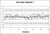
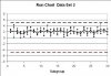
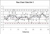
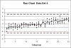
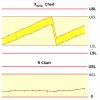
Rather than start with a theoretical presentation of the equations, my plan is to start with the data. In subsequent posts, I will present data for a hypothetical process. Each set of data is generated to illustrate one or more specific features. By seeing the data and the capability indices, hopefully the interpretation will be more concrete, more intuitive.

Unless other wise stated, the following will be true of all the data:

• The process has specification limits at +/- 5
• Data is generated from a normal distribution
• Data are collected into subgroups of 4
• Calculations will be based on 30 subgroups (occasionally 100 subgroups)
• Processing is done with Minitab
• Data will be screened; the data is randomly generated, but data sets that are "too unusual" will be discarded in favor of data that more clearly illustrates the desired features.

I will add data as I have time -- the first few should be available within a few hours as I gather the info and get it posted.

Comments are, of course, welcome. If there are any particular situations you would like illustrated, let me know, and I can try to work it into the series.


Tim

 

[Tim Folkerts]

"Typical" data

Typical Data

This first set of data represents typical data from a process. And by “typical”, I mean “excellent”.

From the run chart, we can see that the data is well centered and well within the specifications. There is definitely variation, but no obvious trends or outliers.

Calculations for this data show

• Cp = 1.61
• Cpk =1.59
• Pp = 1.62
• Ppk = 1.60

All four values are approximately the same, which is apparently one hallmark of an excellent process.


In reality, this data came from a normal distribution random number generator, with a mean of 0 and standard deviation of 1. Theoretically, all four indices should be 1.67. The fact that all are a little smaller than 1.67 can be attributed to random variations. The fact that Cpk is smaller that Cp, and Ppk is slightly smaller than Pp, can be attributed to the mean of the data not being exactly 0.

The random variability of the data was conformed by generating10 different sets of data with the same parameters. In the ten data sets (which should be identical!)

• Cpk varied from 1.41 to 1.80
• Ppk varied from 1.52 to 1.83
• Cpk & Ppk were usually close to each other, but they could be up to about 0.1 different
• Within a given data set, sometimes Cpk > Ppk, and sometimes Ppk > Cpk.
• Variations were reduced when 100 subgroups were used for the calculations

CONCLUSION

• Large, consistent values of the indices indicate excellent data.
• Don’t read too much into small variations between the indices, especially for smaller data sets.

 

[Tim Folkerts]

Data Set 2: a shift in mean

I'm going to forge ahead and insert the images later ...

The second data set shows similar variation, but the center has shifted toward the upper spec limit. I fact, many of the data points are at or outside the specification limits.

Calculations for this data show

• Cp = 1.65
• Cpk = 0.96
• Pp = 1.67
• Ppk = 0.98

(Theoretically, mean = 2, sigma = 1: Cp = Pp = 1.67; Cpk = Ppk = 1.00)

The conclusion is obvious:

• When the center is shifted, Cpk & Ppk are smaller than Cp & Pp.

 

[Tim Folkerts]

Data Set 3: Increased Variation

In this third example, the process is again centered, but the variation has increased.

Calculations for this data show.

• Cp = 0.81
  
• Cpk = 0.79
  
• Pp = 0.80
  
• Ppk = 0.78

(Theoretically, this data has mean = 0, sigma = 2, producing Cp = Cpk = Pp = Ppk = 0.83)

Again, the interpretation is clear and familiar:

• An increase in variation reduces all the capability indices

 

[Tim Folkerts]

Data Set 4: Drift

I wanted to try one slightly more challenging situation.

Here we see that the variation within each group is again similar to Set 1, but there is a significant drift, starting from an average of -2 at the beginning to +2 after 30 subgroups.

The calculations show:

• Cp = 1.65
• Cpk = 1.62
• Pp = 1.12
• Ppk = 1.10
  

(The data has a theoretical mean of 0, a within-subgroup standard deviation of 1.0, and a linear drift from -2 to +2 over the 30 subgroups)

The data is still centered, which agrees with the observation Cp =Cpk, and Pp = Ppk.

This is the first time we have seen Cp ≠ Pp and Cpk ≠ Ppk. Apparently, this is caused by the drift. On other words, when there is some non-random variation (in this case drift) the actual long-term performace (Pp & Ppk) is worse that the short-term potential (Cp & Cpk).




CONCLUSION:

• When there is non-random variation between subgroups, then long-term Pp & Ppk suffer compared to the short-term Cp & Cpk

 

[bobdoering]

Re: Data Set 4: Drift

I wanted to try one slightly more challenging situation.

Here we see that the variation within each group is again similar to Set 1, but there is a significant drift, starting from an average of -2 at the beginning to +2 after 30 subgroups.

The calculations show:

• Cp = 1.65
• Cpk = 1.62
• Pp = 1.12
• Ppk = 1.10
  

(The data has a theoretical mean of 0, a within-subgroup standard deviation of 1.0, and a linear drift from -2 to +2 over the 30 subgroups)

The data is still centered, which agrees with the observation Cp =Cpk, and Pp = Ppk.

This is the first time we have seen Cp ≠ Pp and Cpk ≠ Ppk. Apparently, this is caused by the drift. On other words, when there is some non-random variation (in this case drift) the actual long-term performace (Pp & Ppk) is worse that the short-term potential (Cp & Cpk).




CONCLUSION:

• When there is non-random variation between subgroups, then long-term Pp & Ppk suffer compared to the short-term Cp & Cpk

It seems the assumption is that the drift will continue ad infinitum. If that is the case...maybe so. But, if the system is reset to the lower level and allowed to increase again, as in tool wear, then the game changes. It becomes the sawtooth curve, the uniform distribution, and capability = (USL-LSL)/(UCL-LCL). Also, calculating the averages really has no meaning for that distribution, so plotting the High and Low values of X are much easier and more effective, especially when the origin of this distribution is precision machining.