How to create a pop-up message in Excel

Wanted to have the pop-up message in Excel with the following information:

In a same row the information available is ?Effective date? and the?next review date?.

Wanted the pop-up to be display in 20 days advance.

Is this possible with excel?

Please refer the attachment also.

Thanks.

Re: How to create a pop-up message

Right hand mouse button, select "insert comment". This creates a red, top right corner to the cell which when selected brings out a text box type of callout which you can edit with the text of your choice.

I think this is what you are asking for. It disappears when not on that cell so is useful for giving a bit of info on how to fill a particular box on a form or other type of excel document.

Hope this helps.

Re: How to create a pop-up message

Actually this is probably not what you want. You are looking for something that only appears 20 days before the "review by date" cell. A kind of date triggered alert which only comes up a set number of days before a date in the cell.

That is hard. I am guessing you need some kind of macro to be written. I can not help you there as it requires knowledge of visual basic I think.

I am sure it can be done in excel though by someone with more knowledge than me.

Try conditional formatting. Excel 2010 has a conditional formatting option that will change the cell formatting (background/text color) based on the date in the cell. Excell 2007 probably has this same feature. If you have earlier versions, try subtracting the current date from the cell date and conditional format based on the result.

Try one of these sites:

http://www.mrexcel.com/forum/excel-questions/85556-excel-conditional-popup-message.html

or try a dashboard

http://datapigtechnologies.com/WebinarResources.htm

Miner said:

Try conditional formatting. Excel 2010 has a conditional formatting option that will change the cell formatting (background/text color) based on the date in the cell.

Click to expand...

I agree: That function is what I would (and do) use.

/Claes

Yes conditional formatting in Excel 2003+ (I think) will do this. With older versions you could use a date formula and cell text color or background change to get the same affect, but conditional formatting is much easier.

I don't recall the formula's directly form memory, but if needed could figure them out and post them up fairly quickly. Just let me know.

You can use conditional formatting. Another simple way is simply to use the IF formula. You have effective date in column C and next review date in column D.
In column E, use the following formula:

=IF(D3-TODAY()<=20, "Time for Review", "")

If the next review date is greater than 20 days out, the cell will be blank in column E. If it is less than 20 days, "Time for Review" will print out. You can apply conditional formatting to make it stand out more.

Bill McNeese

raghu_1968 said:

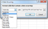
Wanted to have the pop-up message in Excel with the following information:
In a same row the information available is “Effective date” and the”next review date”.
Wanted the pop-up to be display in 20 days advance.

Click to expand...

IMHO, I wouldn't use a pop-up nor conditional formating, I fear of this document could have a few hundred topics.
PopUp bad idea: If several events that need to send the popup, you will be just closing down the popup, witout seeing wich ones send the popup
Conditional formating bad idea if you need to browse across the file to see the colors, nice but not practical....

Better option: A report that make a sheet with the events that need revision (if apply), using VBA, this report can be obtained from clicking a button or entering to the sheet.

I created a button for a respirator fit teting that may work better than a pop up. What this button does it selects based on criteria and it sorts the employees who less than 60 days out from their due date.

I first created conditional formating. Overdue cell is highlighted "red". Less than 60 days is highlighted "yellow"

To create the button:[Developer] [Insert][form controls][Button]

The macro is as follows:

Selection.AutoFilter Field:=5, Criteria1:="<60", Operator:=xlOr, _
Criteria2:="="
Range("C13").Select
Range("C13:G500").Sort Key1:=Range("E14"), Order1:=xlAscending, Header:= _
xlGuess, OrderCustom:=1, MatchCase:=False, Orientation:=xlTopToBottom, _
DataOption1:=xlSortNormal
End Sub

60 is the criteria you will want 20. "C13" is the first cell with data. I used a range of C13-G500. Again the C13 is the first cell with data and G500 is the last.