I have 2 groups to compare - Minitab and stats newbie - Please help

[noorolya.dollah]

Hi
First of all, I am appreciating in advance for those who read this and would like to provide an immediate assistance for my stats issue here.
I have 2 groups to compare; G1 and G2
Each of the group has 6 items to be compared- P1, P2,P3,P4,P5 and P6
There are multiple numbers of subitems in each items, which is in the likert scale of 4 rating , 1-often,2-sometime,3-seldom, 4-never
For example:
P1 ( 5 items)
C1,C2,C3,C4,and C5
I have accumulated 50 samples for each group ; n1=50 and n2=50
Now, my questions are :
1. How do I accumulate/measure the responses or rate in the subitems in each item to find which item has scored the highest in certain group?
For example :
P1=C1+C2+C3+C4+C5=X
P2=C6+C7+C8=Y
I need to compare between these items so that I can make a conclusion that group 1 are more concentrate on the activity of P1 rather than P2.
2. How do I make a comparison between P1 in group 1 and P1 in group 2 to find significant differences between G1 and G2 for each item P1 - P6?
Again, thank you for your help.

 

[Barbara B]

Re: Minitab and stats newbies..please help

Could you please give us the data so we can try for ourselves which analysis could be or should be done? And which Minitab release do you have by hand (Help > About Minitab)?

 

[noorolya.dollah]

Re: Minitab and stats newbies..please help

Hi

Thank you for your prompt response. I am using Minitab 16.

The examples of data as following :

Row C7 C8 C9 C10
1 2 2 2 2
2 2 1 2 2
3 3 3 3 3
4 4 4 4 4
5 2 3 2 3
6 3 1 3 3
7 2 3 3 3
8 4 3 3 4
9 2 1 2 2
10 1 1 1 1
11 2 3 2 3
12 2 2 2 3
13 1 2 2 3
14 1 2 2 3
15 2 3 3 3
16 3 1 3 3
17 3 3 3 2
18 2 1 2 2
19 3 2 3 3
20 3 2 3 3
21 1 2 1 3
22 1 1 1 1
23 1 1 1 2
24 1 2 2 2
25 3 2 2 4
26 3 2 4 4
27 1 3 2 3
28 2 1 1 3
29 3 3 4 3
30 3 3 3 3
31 2 3 2 3
32 2 3 2 3
33 3 2 3 3
34 2 3 2 2
35 3 2 3 3
36 2 3 3 3
37 2 2 2 3
38 2 2 2 2
39 2 3 3 3
40 3 2 3 3
41 2 1 2 2
42 2 1 2 2
43 2 1 1 3
44 2 2 2 3
45 2 3 2 4
46 3 3 3 4
47 3 1 3 3
48 3 2 3 3
49 3 2 3 3
50 2 2 2 3

Please assume that C7 and C8 is in the P1 and C9 and C10 is in the P2.

Thank u so much.

 

[Barbara B]

Re: Minitab and stats newbies..please help

Thanks for the data. I got a little bit lost when trying to figure out which column contains what informations from your first posting, so hopefully my answer is nevertheless helpful.

You can use several different metrics to gather your data for P1, e. g. the sum of the ratings, the mean or the median. To get these row-wise sum for P1 (C7+C8) out of Minitab:
Calc > Row Statistics
Statistic: choose Sum
Input variables: C7 C8
Store result in: 'P1 (sum)'
OK
To get 'P2 (sum)' use the entries in C9 and C10.

First take a look at the data, for example with boxplots:
Graph > Boxplots > Multiple Y's > OK
Graph Variables: 'P1 (sum)' 'P2 (sum)'
OK
They are similar with P2 (sum) being a little bit above P1 (sum), see attached file.

One way to compare the figures could be a 2-sample t-Test, but therefore the data has to follow a normal distribution. To decide which test is appropriate for the comparison between P1 and P2, take a look at the distribution of the numbers
Graph > Probability Plot > Single > OK
Graph Variables: 'P1 (sum)' 'P2 (sum)'
OK
Both graphs show only a handful of different values for P1 (sum) and P2 (sum), so you have not enough evidence to assume that these figures come from a normal distribution. Accordingly the p-value is smaller than 0.005.

The requirements for a t-test are violated. More robust tests with less requirements are nonparametric tests like the Mann-Whitney or Mood-Median-test. They make assumptions about the characteristics in the data, but do not require a specific distribution. E.g. with a Mann-Whitney-test the median of two columns are compared and it is tested whether there is a significant difference between them (see attached file).

For P1 (sum) and P2 (sum) the p-value is 0.0013 and therefore smaller than 0.05 (alpha level). There is only a 0.13% chance to find this difference or a greater difference if in fact both medians are equal, so the difference between P1 (sum) and P2 (sum) is significant.

Hope this helps,

Barbara

 

[noorolya.dollah]

Re: Minitab and stats newbies..please help

Barbara,

Thank you so much for your help.
I have done as suggested, but need to verify some dubious matters.
Here are the steps by step that I followed to analyze my data.

Data examples:

G1 (n=50) G2 (n=50)
6 Main items to be compared with G2:
P1 (8 items) – C23, C36, C37, C41, C42, 43, C44, 45
P2 (5 items) – C24, C27, C34, C39, C40
P3 (3 items) – C25, C32, C33
P4 (5 items) – C26, C28, C31, C38, C46
P5 (2 items) – C30, C35
P6 (3 items) – C29, C47, C48

Data Display

Row C23 C24 C25 C26 C27 C28 C29 C30 C31 C32 C33 C34 C35 C36 C37
1 2 3 3 2 3 3 3 2 2 2 2 3 2 1 2
2 2 1 1 2 2 2 3 1 2 1 2 2 2 2 1
3 2 1 2 4 1 3 4 1 1 1 4 3 1 1 2
4 3 2 1 4 3 4 4 1 3 1 1 4 4 1 3
5 3 2 1 2 1 2 2 1 1 1 1 2 2 1 1
6 2 1 3 3 1 3 4 1 2 2 3 3 1 2 2
7 2 2 2 2 2 2 2 1 2 1 2 2 2 1 1
8 3 3 2 4 3 3 4 2 2 2 1 2 2 1 1
9 1 1 1 2 1 2 2 1 1 1 1 1 1 1 1
10 1 1 1 1 1 1 1 1 1 1 1 1 1 1 1
11 2 2 2 1 2 3 3 1 2 2 3 4 4 2 1
12 2 1 2 2 2 2 3 1 1 2 3 2 3 2 2
13 1 1 1 1 1 1 1 1 1 1 3 1 2 1 1
14 1 1 1 1 1 1 1 1 1 1 3 1 2 1 1
15 2 2 3 2 3 2 3 1 2 1 3 3 3 2 2
16 1 1 2 3 1 3 3 1 2 1 3 2 3 3 3
17 2 2 2 2 3 3 3 1 3 2 4 3 3 3 3
18 1 1 2 1 1 2 2 1 1 1 2 1 1 1 1
19 3 2 3 3 1 3 3 2 2 2 3 3 3 3 3
20 2 2 2 2 2 2 2 3 2 2 2 2 2 3 2
21 1 1 2 1 1 1 2 1 1 1 1 3 3 2 1
22 1 1 1 1 1 1 1 1 1 1 1 1 1 1 1
23 1 1 1 1 1 2 2 1 1 1 1 1 1 1 1
24 2 1 1 2 2 3 2 1 2 1 2 2 2 2 1
25 4 4 3 4 1 4 4 1 2 1 3 3 1 2 3
26 1 1 1 1 1 3 4 1 3 2 3 4 4 3 1
27 2 2 2 1 1 2 3 2 2 1 4 2 4 1 1
28 3 2 3 2 1 1 3 1 3 1 1 3 3 1 1
29 2 3 2 4 3 4 3 2 3 2 2 2 3 3 3
30 2 2 3 4 2 3 2 1 2 3 3 3 3 2 2
31 2 2 2 3 2 2 2 2 2 2 1 3 3 2 1
32 2 2 1 2 3 2 3 1 3 3 3 3 3 2 2
33 1 1 2 1 2 2 3 1 1 1 1 1 2 2 1
34 2 2 3 3 2 3 3 2 2 3 3 3 3 2 2
35 1 1 3 3 2 1 2 2 2 2 3 2 3 1 1
36 1 1 2 1 2 2 2 2 2 2 2 2 3 2 2
37 3 3 2 3 2 3 3 3 2 2 3 3 3 2 3
38 1 1 1 2 1 2 2 1 2 1 3 1 1 2 1
39 2 2 3 3 2 3 3 2 2 1 4 2 2 2 2
40 3 2 3 4 3 3 3 1 1 1 4 4 3 3 1
41 2 2 2 2 1 2 2 1 2 1 3 2 3 1 2
42 2 1 3 3 1 2 3 3 2 2 3 4 4 2 1
43 1 2 3 2 1 2 4 2 2 1 3 3 3 2 2
44 2 2 2 2 2 2 2 2 2 2 2 2 2 2 2
45 1 1 2 2 2 1 1 1 1 1 1 1 1 1 1
46 1 2 3 3 3 3 3 2 3 2 3 4 3 3 2
47 1 1 2 3 2 3 3 1 2 1 1 2 2 3 2
48 1 1 * 3 1 3 3 1 1 1 * 3 3 1 1
49 2 3 2 3 2 3 3 2 3 1 1 2 3 3 2
50 1 1 2 1 2 2 2 1 2 1 1 1 1 1 1

Row C38 C39 C40 C41 C42 C43 C44 C45 C46 C47 C48
1 2 3 2 1 1 1 2 2 2 3 2
2 1 1 1 1 1 2 2 1 1 2 2
3 1 4 1 1 1 3 2 2 1 4 2
4 1 3 1 2 1 1 1 1 1 3 3
5 1 1 1 1 1 1 2 1 1 2 2
6 2 3 1 1 1 2 2 2 1 3 1
7 1 1 2 2 1 2 2 1 1 1 1
8 1 2 2 1 3 1 1 1 1 2 1
9 1 2 1 1 1 1 2 1 1 2 1
10 1 1 1 1 1 2 2 1 1 2 1
11 3 2 2 2 1 1 1 1 1 3 1
12 2 1 2 2 2 2 2 2 2 3 2
13 1 1 1 1 1 1 1 2 1 2 1
14 1 1 1 1 1 1 1 2 1 2 1
15 2 3 1 2 2 2 2 2 1 3 2
16 3 3 1 2 1 2 2 2 2 3 3
17 2 2 1 3 2 1 1 2 1 2 1
18 1 2 1 1 1 2 1 1 1 1 1
19 2 1 1 1 2 3 1 1 1 3 3
20 2 2 3 2 2 2 2 2 2 2 2
21 2 2 1 1 2 1 1 1 1 2 2
22 1 1 1 1 1 1 1 1 1 1 1
23 2 1 1 1 1 1 1 1 1 2 1
24 1 2 1 1 1 2 2 2 2 2 3
25 3 3 2 2 2 2 4 2 2 4 3
26 3 1 2 3 1 2 2 2 2 2 2
27 1 3 2 1 1 2 1 2 1 2 2
28 1 3 1 1 1 2 1 1 1 3 1
29 3 2 2 2 2 3 3 1 2 3 3
30 3 3 2 1 2 2 2 2 2 3 3
31 1 2 3 1 1 1 2 1 1 1 1
32 2 2 1 1 2 2 2 2 2 2 2
33 * 1 1 1 1 1 2 1 1 2 2
34 1 1 1 1 3 1 3 1 1 3 2
35 1 1 2 1 2 1 1 1 2 1 2
36 1 1 1 2 1 2 3 2 1 2 2
37 2 3 3 2 2 2 3 3 2 3 3
38 2 2 1 1 1 2 1 2 1 2 1
39 2 2 2 2 2 2 3 3 2 3 2
40 3 4 1 1 1 3 3 3 1 4 3
41 1 2 2 1 1 2 2 1 1 2 1
42 1 3 1 1 2 1 2 1 1 3 3
43 3 2 1 1 1 1 2 1 1 2 1
44 2 2 2 2 2 2 2 2 2 2 2
45 1 2 1 1 1 2 1 1 1 2 1
46 2 3 1 1 2 2 2 3 2 2 3
47 2 1 1 1 1 2 1 1 1 2 1
48 * 1 1 2 2 1 3 1 2 1 3
49 3 2 1 1 1 2 1 2 1 3 1
50 1 2 2 2 1 1 1 1 1 1 1




Steps that I have done:

• As the data is in the likert scale : 1-often,2-sometime,3-seldom, 4-never, so I think I should changed it based on numbers that reflect on the option chosen by the samples, which means if they choose 1 or 2 , it will be more to positive one and 3 or 4 not so positive. I have changed it based on the marking score
• : 1=4 mark, 2=3 mark, 3=2 mark, 4=1 mark by using Data> Code> Numeric to Numeric and change it accordingly:

Code data from columns = C23 – C48
Store coded data in columns= C23 –C48
Original values New
1 4
2 3
3 2
4 1

Click OK.

• Then, I do the sum of rating as suggested.

P1 (C23+C36+C41+C42+C43+C44+C45) = ‘Type1 (sum)’
P2 (C24+C27+C34+C39+C40) = ‘Type2 (sum)’
P3 (C25+C32+C33) = ‘Type3 (sum)’
P4 (C26+C28+C31+C38+C46) = ‘Type 4(sum)’
P5 (C30+C35) = ‘Type 5(sum)’
P6 (C29+C47+C48) = ‘Type 6 (sum)’

• Once I got the values in the column, I did a box plot as attached.
• However, I am struggling to write a description for this box plot. I know the middle line is the median, but I am still can’t figure out how to describe this data. My assumption when I look at this boxplot, Type1 or P1 has scored the highest among all and Type 5 or P5 is the lowest.
• I did the same steps to a set of data in G2 and attached is the boxplot as well. Again, please help me to describe the data.
• I have been advised by my supervisor that would be easier to understand if I may convert the score of P1-P6 to percentages. So, here what I did; I calculate the expected highest score for each main item using this formula :

highest mark(4) x number of subitems (Y) x number of samples
So, I’ve got this value for each of the item:
P1 = 4 x 8x 50 = 1600
P2 = 4 x 5 x 50 = 1000
P3 = 4 x 3 x 50 = 600
P4 = 4 x 5 x 50 = 1000
P5 = 4 x 2 x 50 = 400
P6 = 4 x 3 x 50 = 600

• Then, I total up each of the main item using Column statistics and got the value below:

Type 1 (total) = 1348
Type 2 (total) = 793
Type 3 (total) = 455
Type 4 (total) = 768
Type 5 (total) = 310
Type 6 (total) = 413

• Since I am not sure how to do this in the minitab, so I did the following steps manually, which to get the percentage of each item by using this formula :

Total / expected highest score x 100
and here are the percentages that derived from that values:

Type 1 = 1348/1600 x 100 = 84.25%
Type 2 = 793/1000 x 100 = 79.3 %
Type 3 = 455/600 x 100 = 75.8%
Type 4 = 768/1000 x 100 = 76.8 %
Type 5 = 310/400 x 100 = 77.5 %
Type 6 = 413/600 x 100 = 68.8 %



As a first glance, it showed that Type 1 scored the highest as equivalent with the boxplot result, but it is contradict with the lowest score, which is scored by Type 6 instead of Type 5 in the box plot result. Please advise.

• As for comparison, below is the actual data that I have to compare between G1 and G2.

Group 1 (G1)
Type1 Type2 Type3 Type4 Type5 Type6
Row (sum) (sum) (sum) (sum) (sum) (sum)
1 28 11 8 14 6 7
2 28 18 11 17 7 8
3 26 15 8 15 8 5
4 27 12 12 12 5 5
5 29 18 12 18 7 9
6 26 16 7 14 8 7
7 28 16 10 17 7 11
8 28 13 10 14 6 8
9 31 19 12 18 8 10
10 30 20 12 20 8 11
11 29 13 8 15 5 8
12 24 17 8 16 6 7
13 31 20 10 20 7 11
14 31 20 10 20 7 11
15 24 13 8 16 6 7
16 24 17 9 12 6 6
17 23 14 7 14 6 9
18 31 19 10 19 8 11
19 23 17 7 14 5 6
20 23 14 9 15 5 9
21 30 17 11 19 6 9
22 32 20 12 20 8 12
23 32 20 12 18 8 10
24 27 17 11 15 7 8
25 19 12 8 10 8 4
26 25 16 9 13 5 7
27 29 15 8 18 4 8
28 29 15 10 17 6 8
29 21 13 9 9 5 6
30 25 13 6 11 6 7
31 29 13 10 16 5 11
32 25 14 8 14 6 8
33 30 19 11 15 7 8
34 25 16 6 15 5 7
35 31 17 7 16 5 10
36 25 18 9 18 5 9
37 20 11 8 13 4 6
38 29 19 10 16 8 10
39 22 15 7 13 6 7
40 22 11 7 13 6 5
41 28 16 9 17 6 10
42 28 15 7 16 3 6
43 29 16 8 15 5 8
44 24 15 9 15 6 9
45 31 18 11 19 8 11
46 24 12 7 12 5 7
47 28 18 11 14 7 9
48 28 18 4 11 6 8
49 26 15 11 12 5 8
50 31 17 11 18 8 11

Group 2 ( G2)
Data Display

Type Type Type Type Type Type
1-G2 2-G2 3-G2 4-G2 5-G2 6-G2
Row (sum) (sum) (sum) (sum) (sum) (sum)
1 29 18 4 15 3 11
2 30 20 6 14 2 9
3 29 17 6 16 3 8
4 30 19 8 17 2 11
5 26 17 6 14 4 6
6 22 15 5 10 2 3
7 31 20 12 17 6 9
8 31 18 7 11 3 8
9 32 20 12 15 6 11
10 28 18 7 14 6 9
11 31 20 8 18 5 9
12 25 17 7 15 2 7
13 29 20 12 19 7 11
14 26 18 11 14 7 8
15 22 14 6 9 3 5
16 32 18 10 19 8 12
17 30 15 3 13 3 6
18 30 18 6 13 3 7
19 25 16 7 15 2 9
20 31 20 9 17 4 9
21 24 14 8 12 5 8
22 31 18 6 16 4 6
23 25 18 9 16 3 5
24 30 14 6 15 2 6
25 28 20 7 11 5 7
26 3 9 10 7 3 *
27 32 20 10 18 5 12
28 30 19 9 15 5 8
29 31 19 7 16 6 7
30 27 17 7 12 2 6
31 26 16 9 16 4 10
32 26 17 11 14 6 9
33 26 19 10 11 6 9
34 24 20 10 16 5 10
35 32 20 9 14 2 4
36 32 19 12 15 7 8
37 26 15 6 17 3 7
38 32 20 12 20 8 12
39 31 20 12 17 7 11
40 27 17 10 15 3 7
41 30 17 9 17 2 7
42 30 20 11 16 3 9
43 26 15 7 15 4 6
44 28 18 6 15 4 8
45 30 14 4 16 8 7
46 26 13 6 12 2 6
47 31 19 11 16 6 11
48 24 17 7 13 2 3
49 22 19 8 13 2 7
50 27 19 5 20 2 11

• I have done normality test for each items to compare and attached the result in the normality test file.
• As all items have formed a straight line, so may I assume all data in each items are normally distributed?
• Based on my assumption of the normality test, I have done 2-t-test as suggested and here are the results.

Two-Sample T-Test and CI: Type1 (sum), Type 1-G2 (sum)

Two-sample T for Type1 (sum) vs Type 1-G2 (sum)

N Mean StDev SE Mean
Type1 (sum) 50 26.96 3.32 0.47
Type 1-G2 (sum) 50 27.72 4.62 0.65


Difference = mu (Type1 (sum)) - mu (Type 1-G2 (sum))
Estimate for difference: -0.760
95% CI for difference: (-2.359, 0.839)
T-Test of difference = 0 (vs not =): T-Value = -0.94 P-Value = 0.347 DF = 88

Two-Sample T-Test and CI: Type2 (sum), Type 2-G2 (sum)

Two-sample T for Type2 (sum) vs Type 2-G2 (sum)

N Mean StDev SE Mean
Type2 (sum) 50 15.86 2.64 0.37
Type 2-G2 (sum) 50 17.60 2.36 0.33


Difference = mu (Type2 (sum)) - mu (Type 2-G2 (sum))
Estimate for difference: -1.740
95% CI for difference: (-2.735, -0.745)
T-Test of difference = 0 (vs not =): T-Value = -3.47 P-Value = 0.001 DF = 96

Two-Sample T-Test and CI: Type3 (sum), Type 3-G2 (sum)

Two-sample T for Type3 (sum) vs Type 3-G2 (sum)

N Mean StDev SE Mean
Type3 (sum) 50 9.10 1.91 0.27
Type 3-G2 (sum) 50 8.12 2.41 0.34


Difference = mu (Type3 (sum)) - mu (Type 3-G2 (sum))
Estimate for difference: 0.980
95% CI for difference: (0.116, 1.844)
T-Test of difference = 0 (vs not =): T-Value = 2.25 P-Value = 0.027 DF = 93


Two-Sample T-Test and CI: Type4 (sum), Type 4-G2 (sum)

Two-sample T for Type4 (sum) vs Type 4-G2 (sum)

N Mean StDev SE Mean
Type4 (sum) 50 15.36 2.75 0.39
Type 4-G2 (sum) 50 14.82 2.69 0.38


Difference = mu (Type4 (sum)) - mu (Type 4-G2 (sum))
Estimate for difference: 0.540
95% CI for difference: (-0.538, 1.618)
T-Test of difference = 0 (vs not =): T-Value = 0.99 P-Value = 0.323 DF = 97


Two-Sample T-Test and CI: Type5 (sum), Type 5-G2 (sum)

Two-sample T for Type5 (sum) vs Type 5-G2 (sum)

N Mean StDev SE Mean
Type5 (sum) 50 6.20 1.28 0.18
Type 5-G2 (sum) 50 4.14 1.92 0.27


Difference = mu (Type5 (sum)) - mu (Type 5-G2 (sum))
Estimate for difference: 2.060
95% CI for difference: (1.412, 2.708)
T-Test of difference = 0 (vs not =): T-Value = 6.32 P-Value = 0.000 DF = 85


Two-Sample T-Test and CI: Type6 (sum), Type 6-G2 (sum)

Two-sample T for Type6 (sum) vs Type 6-G2 (sum)

N Mean StDev SE Mean
Type6 (sum) 50 8.26 1.94 0.27
Type 6-G2 (sum) 49 8.06 2.28 0.33


Difference = mu (Type6 (sum)) - mu (Type 6-G2 (sum))
Estimate for difference: 0.199
95% CI for difference: (-0.645, 1.043)
T-Test of difference = 0 (vs not =): T-Value = 0.47 P-Value = 0.641 DF = 93


Again, I am struggling here to interpret the result. Please help.

My supervisor has also suggested for me to use ANOVA for comparison. Do you think it would be sufficient using t-test or should I further analysis using ANOVA as per advised?

Appreciate your help and thanking you in advance.

 

[Barbara B]

Re: Minitab and stats newbies..please help

• Then, I do the sum of rating as suggested.

P1 (C23+C36+C41+C42+C43+C44+C45) = ‘Type1 (sum)’
P2 (C24+C27+C34+C39+C40) = ‘Type2 (sum)’
P3 (C25+C32+C33) = ‘Type3 (sum)’
P4 (C26+C28+C31+C38+C46) = ‘Type 4(sum)’
P5 (C30+C35) = ‘Type 5(sum)’
P6 (C29+C47+C48) = ‘Type 6 (sum)’

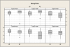
• Once I got the values in the column, I did a box plot as attached.
• However, I am struggling to write a description for this box plot. I know the middle line is the median, but I am still can’t figure out how to describe this data. My assumption when I look at this boxplot, Type1 or P1 has scored the highest among all and Type 5 or P5 is the lowest.
• I did the same steps to a set of data in G2 and attached is the boxplot as well. Again, please help me to describe the data.

If you take the sum of the ratings, the sums for P1 will usually be higher because you sum up 7 ratings and the sums for P5 will be lower because you sum up only 2 ratings. So even if the P5 ratings are high (e. g. 4 and 4) the sum will only be 8. For P1 with mid-high ratings (e. g. 2,3,3,2,1,2 and 3) the sum is 16. (Note: In your formula for Type 1 (sum) you have only 7 ratings C23+C36+C41+C42+C43+C44+C45 for P1, but in the formula for the percentages are 8 ratings or subitems.)

To get comparable numbers you have to divide the sum with a figure which reflects the number of items in the sum. One approach is to use the mean (sum/ (no. of subitems)), another the calculation of a percentage value advised by your supervisor (sum / (highest mark*no. of subitems*sample size)).

To calculate this or other formulas in Minitab you could use the calculator with several build-in function similar to those in Excel:
Calc > Calculator
Store result in variables: Type 1 (%)
Expression: 'Type1'/1600*100
OK

I calculated the means of your G1 and G2 data as follows:
'Type1 mean' = 'Type1'/8
'Type2 mean' = 'Type2'/5
'Type3 mean' = 'Type3'/3
'Type4 mean' = 'Type4'/5
'Type5 mean' = 'Type5'/2
'Type6 mean' = 'Type6'/3
(sum / no.of.subitems)

The boxplots seem to be similar for all 6 types (see data and graph attached).

• I have done normality test for each items to compare and attached the result in the normality test file.
• As all items have formed a straight line, so may I assume all data in each items are normally distributed?
• ...

The variation in your ratings is too small to see a normal distribution in the data. Due to the small amount of different values (either in the sum, mean or percentage) you get stacked points in the probability plot and therefore a violation of the normality assumption.

The Anderson-Darling test for normality (AD-test) shown in the legend on the right side of each graph detects almost always a significant deviation from the normal assumption (p-value <0.05 = data not normally distributed), so you could not use a t Test and get reliable results in the comparison of G1 and G2. A nonparametric test is recommended here.

• Based on my assumption of the normality test, I have done 2-t-test as suggested and here are the results.

Two-Sample T-Test and CI: Type1 (sum), Type 1-G2 (sum)

Two-sample T for Type1 (sum) vs Type 1-G2 (sum)

N Mean StDev SE Mean
Type1 (sum) 50 26.96 3.32 0.47
Type 1-G2 (sum) 50 27.72 4.62 0.65


Difference = mu (Type1 (sum)) - mu (Type 1-G2 (sum))
Estimate for difference: -0.760
95% CI for difference: (-2.359, 0.839)
T-Test of difference = 0 (vs not =): T-Value = -0.94 P-Value = 0.347 DF = 88
[...]

Again, I am struggling here to interpret the result. Please help.

The 2t-test looks for differences between two means, here: mean of Type1-G1(sum) and mean of Type1-G2(sum). This difference is calculated as
26.96-27.72=-0.760

The p-value gives the probability to find this difference (or a higher one) in the data, if the means of G1 and G2 are in fact equal (H0 assumption). The p-value for the difference between mean of G1 and G2 is given as p=0.347 >0.05, so it could be interpreted as "no significant difference between G1 and G2 in the type 1 ratings", but the normality assumption isn't met for the data.

If your values for G1 and G2 are in different columns, you could use the nonparametric Mann-Whitney test to evaluate if the medians of G1 and G2 are different. (If your data is in one column and the grouping factor in another like in the spreadsheet attached, you could use the Kruskal-Wallis test instead. The Mann-Whitney test is the same as the Kruskal-Wallis test for 2 groups.)

Mann-Whitney Test and CI: Type1 mean_G1; Type1 mean_G2

N Median
Type1 mean_G1 50 3.5000
Type1 mean_G2 50 3.6250

Point estimate for ETA1-ETA2 is -0.1250
95,0 Percent CI for ETA1-ETA2 is (-0.2500;-0.0001)
W = 2273.0
Test of ETA1 = ETA2 vs ETA1 not = ETA2 is significant at 0.0830
The test is significant at 0.0813 (adjusted for ties)


"ETA1" is the median of Type1 for G1 and "ETA2" the median for G2. The p-value in the Mann-Whitney test is the probability to get this difference (or a higher one) in the data if the medians of both samples are in fact the same. The p-value obtained for Type1 in G1 and G2 is p=0.0830 or rather p=0.0813 (ties occur due to equal values in the sample, so the later is the more appropriate p-value). p is greater than 0.05 so there is not enough evidence in the data to assume that a significant difference exist between Type1 in G1 and G2.

My supervisor has also suggested for me to use ANOVA for comparison. Do you think it would be sufficient using t-test or should I further analysis using ANOVA as per advised?

You'll get a lot more informations out of an ANOVA than test procedures could provide, but the complexity of the analysis will increase just as well. Here are some opportunities provides with ANOVA:
*Evaluation of interactions (e.g. Type & Group)
*Evaluation of model quality: Which amount of variability in the data could be assigned to the factors in the model? (R-Sq, R-Sq(adj))
*Comparisons and multiple comparisons of levels (e.g. Tukey, Bonferroni)
*Detection of extreme values and outliers not explained due to factor settings (residual plot)

Due to missing values you have to use the GLM out of the ANOVA menu (Two-way ANOVA will only work for equal numbers of items in every subgroup, that is in a balanced design):
Stat > ANOVA > GLM
Responses: 'mean ratings'
Model: Group Type Group*Type
Group (G1/G2), Type (Type1-Type6) and interaction Group*Type are included in the ANOVA model
> Graphs:
Residual Plots: Choose "Four in one"
OK
> Factor Plots:
Main Effect Plot: Factor: Group Type
Interaction Plot: Factor: Group Type [without asterisk!]
OK
> Comparisons:
Terms: Group Type
Method: Tukey, choose "Grouping information", "Confidence Interval", "Test"
OK > OK

Take a look at the results and decide for yourself if it't worth to struggle with it or if you want to stick to the tests instead.

Best regards,

Barbara

 

[Miner]

One point of caution in addition to Barbara's excellent comments.

You are performing 6 t-Tests above. While the probability of a specious false positive is only 0.05 for a single t-Test, the probability of one for 6 tests is 1-0.96^6 = 0.26, or a 1 in 4 chance. You should use a post-hoc Multiple comparisons approach such as Tukey's HSD to control the family error rate. Minitab offers a number of these packaged with the ANOVA routines.

 

[noorolya.dollah]

Re: Minitab and stats newbies..please help

Hi Barbara,

Thank you so much for you help. I am working on it now.
Btw, just want to inform you that I only got one file from your posted attachement.
Would you mind to reattach the files as mentioned in your comment,

The boxplots seem to be similar for all 6 types (see data and graph attached).

Thanks again.

 

[Barbara B]

Re: Minitab and stats newbies..please help

Sorry for the lost attachements, hope this works now

 

[noorolya.dollah]

Re: Minitab and stats newbies..please help

Good day Barbara,

I have done all the steps as suggested and here are some of my dubious matters:

• I have chosen both methods: mean score (sum/item) and percentages (total/expected highest score x 100) to represent the data comparison of 6 main items (P1, P2, P3, P4, P5 and P6) in each group.(note for P1-it is 8 items as I left to add C37 in). I have attached the table as i plan to attach in my report. However, how do I use minitab to represent the percentages of data for main items in each group in the graphical mode-for better understanding?
• For comparison between G1 and G2, I have tried to use ANOVA>GLM based on the data given. You are right! There are lots of complexities going on for me to interpret the data right now. Take a look on the result and my assumption as attached. Please correct me if I am wrong on the data interpretation.
• Please advise me further on the steps to get to this result as well. I need to understand right from the start when you extract the data into the table that you attached to me in your reply before.

Again, thank you very much for your kind support. Really appreciate it!